For my September 2021 diary, go here.

Diary — October 2021

John Baez

I think this print is by Takeji Asano. The glowing lights in the houses and especially the boat are very inviting amid the darkness. You want to go inside.

October 3, 2021

I'll use 'ring' to mean 'commutative ring'.

The continuous real-valued functions on a topological space form a ring $C(X)$, and the functions that vanish at one point form a maximal ideal $M$ in this ring. This makes us want 'points' of a ring to be maximal ideals.

Indeed, it's all very nice: $C(X)/M$ is isomorphic to the complex numbers $\mathbb{C}$, and the quotient map $$C(X)\to C(X)/M\cong \mathbb{C}$$ is just evaluating a function at a point.

Even better, if $X$ is a compact space every maximal ideal $M\subset C(X)$ consists of functions that vanish at some point in $X$. If furthermore $X$ is also Hausdorff, the choice of this point is unique.

In short, points of a compact Hausdorff space $X$ are just the same as maximal ideals of $C(X)$. So we have captured, using just algebra, the concept of 'point' and 'evaluating a function at a point'.

The problem starts when we try to generalize from $C(X)$ to other commutative rings.

At first all seems fine: for any ideal $J$ in any ring $R$, the quotient $R/J$ is a field if and only if $J$ is maximal. And we like fields — since we learned linear algebra using fields.

But then the trouble starts. Any continuous map of spaces $X\to Y$ gives a ring homomorphism $C(Y)\to C(X)$. This is the grand duality between topology and commutative algebra! So we'd like to run it backwards: for any ring homomorphism $R\to S$ we a map sending 'points' of $S$ to 'points' of $R$.

But if we define 'points' to be maximal ideals it doesn't work. Given a homomorphism $f:R\to S$ and a maximal ideal $M$ of $S$, the inverse image $f^{-1}(M)$ is an ideal of $R$, but not necessarily a maximal ideal!

Why not?

To tell if an ideal is maximal you have to run around comparing it with all other ideals! This depends not just on the ideal itself, but on its 'environment'. So $M$ being maximal doesn't imply that $f^{-1}(M)$, living in a completely different ring, is maximal.

In short, the logic we're using to define 'maximal ideal' is too complex! We are quantifying over all ideals in the ring, so the concept we're getting is very sensitive to the whole ring — so maximal ideals don't transform nicely under ring homomorphisms.

It turns out prime ideals are much better. An ideal $P$ is prime if it's not the whole ring and $ab\in P$ implies $a\in P$ or $b\in P$.

Now things work fine: given a homomorphism $f:R\to S$ and a prime ideal $P$ of $S$, the inverse image $f^{-1}(P)$ is a prime ideal of $R$.

Why do prime ideals work where maximal ideals failed?

It's because checking to see if an ideal is prime mainly involves checking things within the ideal — not its environment! None of this silly running around comparing it to all other ideals.

And we also get a substitute for our beloved fields: integral domains. An integral domain is a ring where if $ab=0$, then either $a=0$ or $b=0$. For any ideal $J$ in any ring $R$, the quotient $R/J$ is an integral domain if and only if $J$ is a prime ideal. This theorem is insanely easy to prove!

So: by giving up our attachment to fields, we can work with concepts that are logically simpler and thus 'more functorial'. We get a contravariant functor from rings to sets, sending each ring to its set of prime ideals.

With maximal ideals, life is much more complicated and messy.

October 4, 2021

Why weird? Only because I'd been avoiding this sort of math until now. For some reason I took a dislike to commutative algebra as a youth. Dumb kid.

I liked stuff I could visualize so I liked the idea of a vector bundle: a bunch of vector spaces, one for each point in a topological space $X$, varying continuously from point to point. If you 'localize' a vector bundle at a point you get a vector space.

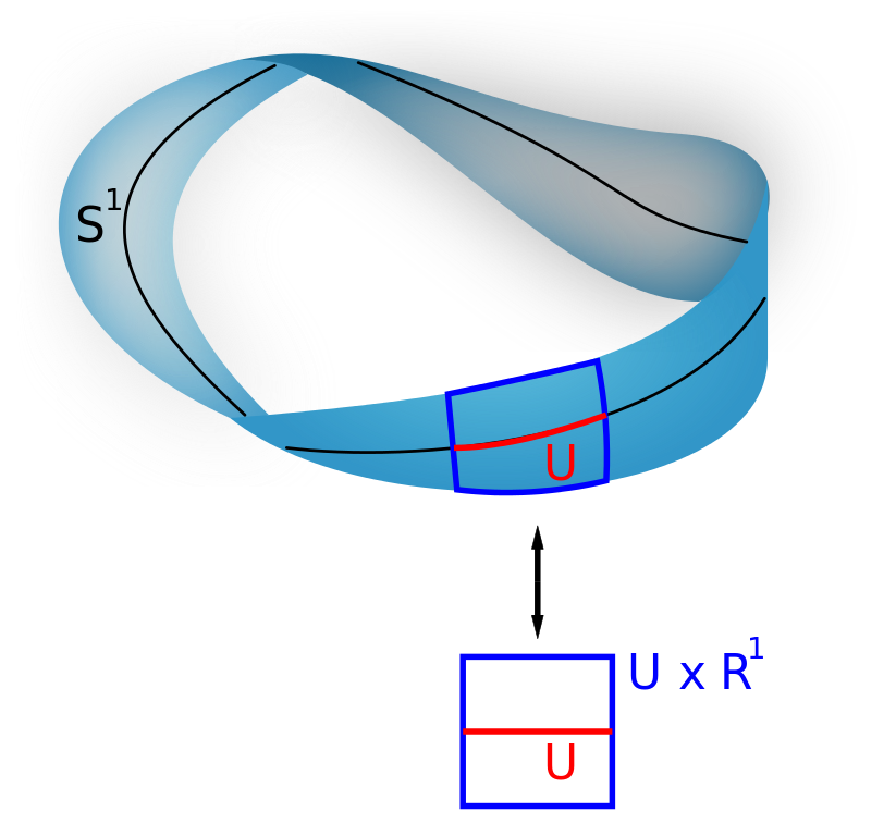
In this example the vector bundle is the Möbius strip. The space $X$ is the circle $S^1$, and the vector space at each point is the line ${\mathbb{R}}^1$. If you restrict attention to a little open set $U$ near a point, the Möbius strip looks like $U\times {\mathbb{R}}^1$. So, you can say that localizing this vector bundle at any point gives ${\mathbb{R}}^1$.

But this nice easy-to-visualize stuff is also commutative algebra! For any compact Hausdorff space $X$, the continuous complex-valued functions on it, $C(X)$, form a kind of commutative ring called a 'commutative C*-algebra'. And any commutative C*-algebra comes from some compact Hausdorff space $X$. This fact is called the Gelfand-Naimark theorem.

(I liked this sort of commutative algebra because it involved a lot of things like I knew how to visualize, like topology and analysis. Also, C*-algebras describe the observables in classical and quantum systems, with commutative ones describing the classical ones.)

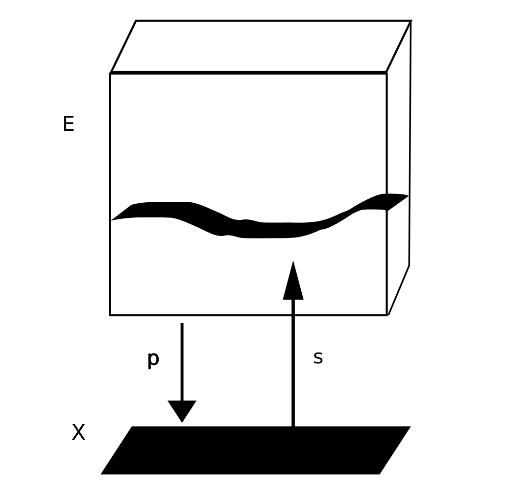
Now, given a vector bundle over $X$, like $E$ here, its 'sections', like $s$ here, form a module of the commutative ring $C(X)$. And not just any sort of module: you get a 'finitely generated projective module'. (These are buzzwords that algebraists love.)

Again, we can turn this around: every finitely generated projective module of $C(X)$ comes from a vector bundle over $X$. This is called 'Swan's theorem'.

So: whenever someone says 'finitely generated projective module over a commutative ring' I think 'vector bundle' and see this:

But to get this mental image to really do work for me, I had to learn how to 'localize' a projective module of a commutative ring 'at a point' and get something kind of like a vector space. And then I had to learn a bunch of basic theorems, so I could use this technology.

I could have learned this stuff in school like the other kids. I've sort of read about it anyway — you can't really avoid this stuff if you're in the math biz. But actually needing to do something with it radically increased my enthusiasm!

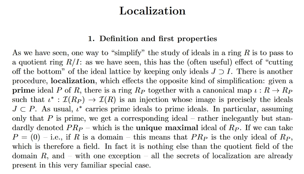
For example, I was suddenly delighted by Kaplansky's theorem. The analogue of a 'point' for a commutative ring $R$ is a prime ideal: an ideal $\mathfrak{p}\subset R$ that's not the whole ring such that $ab\in \mathfrak{p}$ implies either $a\in \mathfrak{p}$ or $b\in \mathfrak{p}$. We localize a ring $R$ at the prime ideal $\mathfrak{p}$ by throwing in formal inverses for all elements not in $\mathfrak{p}$. The result, called $R_{\mathfrak{p}}$, is a local ring, meaning a ring with just one maximal ideal.

When you do this, any module $M$ of $R$ gives a module $M_{\mathfrak{p}}$ of the localization of $R$. And Kaplansky's theorem says that any projective module of $R$ gives a free module of that local ring. This is a lot like a vector space over a field! After all, any vector space is a free module: this is just a fancy way of saying it has a basis.

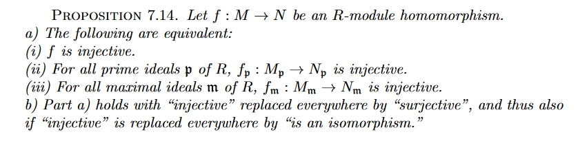
Furthermore, a map between of modules of a commutative ring R has an inverse iff it's true 'localized at each point'. Just like a map between vector bundles over $X$ has an inverse iff the map between vector spaces it gives at each point of $X$ has an inverse!

I know all the algebraic geometers are laughing at me like a 60-year-old who just learned how to ride a tricycle and is gleefully rolling around the neighborhood. But too bad! It's never too late to have some fun!

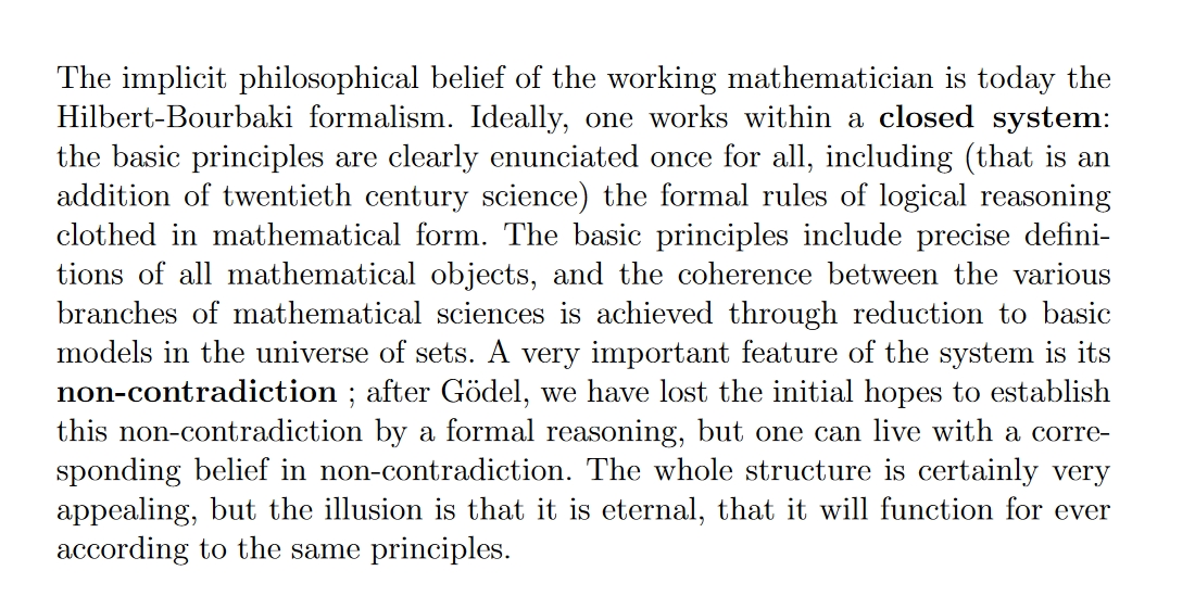
By the way, the quotes above come from this free book, which I'm enjoying now:

• Pete L. Clark, Commutative Algebra.

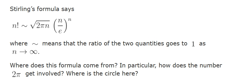
Stirling's formula gives a good approximation of the factorial $$n!=1\times 2\times 3\times \cdots \times n$$ It's obvious that $n!$ is smaller than $$n^n=n\times n\times n\times \cdots \times n$$ But where do the $e$ and $\sqrt{2\pi }$ come from?

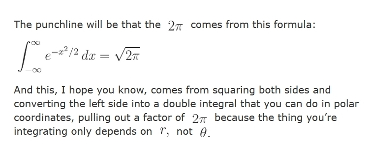
The easiest way to see where the $\sqrt{2\pi }$ comes from is to find an integral that equals n! and then approximate it with a 'Gaussian integral', shown below.

This is famous: when you square it, you get an integral with circular symmetry, and the $2\pi$ pops right out!

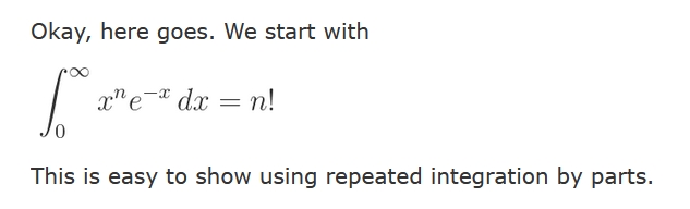
But how do you get an integral that equals $n$ factorial? Try integrating $x^n$ times an exponential! You have to integrate this by parts repeatedly. Each time you do, the power of $x$ goes down by one and you can pull out the exponent: first $n$, then $n-1$, then $n-2$, etc.

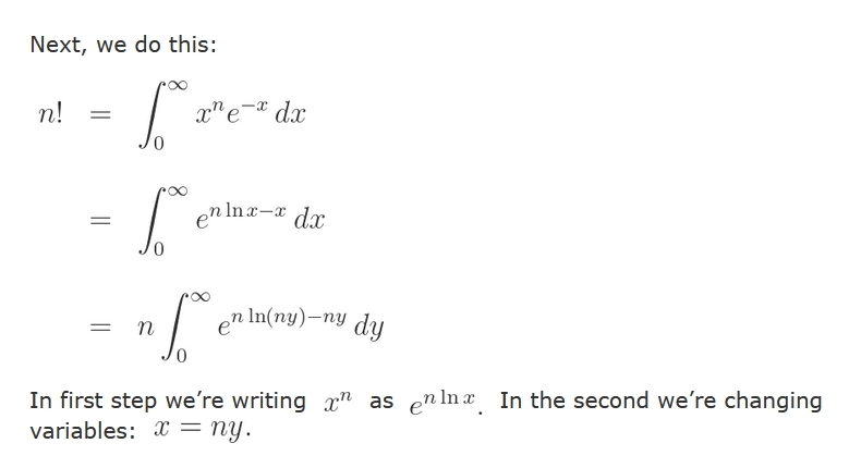
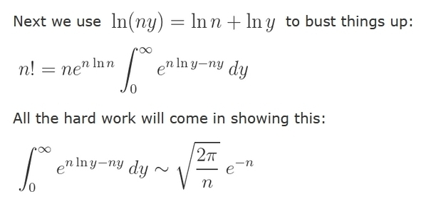
Next, write $x^n$ as \(e^{n \ln x|\). With a little cleverness, this gives a formula for n! that's an integral of $e$ to $n$ times something. This is good for seeing what happens as $n\to \mathrm{\infty }$.

There's just one problem: the 'something' also involves $n$: it contains $\ln (ny)$.

But we can solve this problem by writing $\ln (ny)=\ln n+\ln y$. With a little fiddling this gives an integral of $e$ to $n$ times something that doesn't depend on $n$. Then, as we take $n\to \mathrm{\infty }$, this will approach a Gaussian integral. And that's why $\sqrt{2\pi }$ shows up!

Oh yeah — but what about proving Stirling's formula? Don't worry, this will be easy if we can do the hard work of approximating that integral. It's just a bit of algebra:

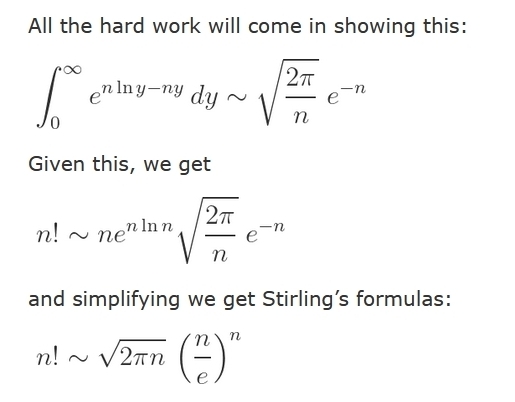
So, this proof of Stirling's formula has a 'soft outer layer' and a 'hard inner core'. First you did a bunch of calculus tricks. But now you need to take the $n\to \mathrm{\infty }$ limit of the integral of $e$ to $n$ times some function.

Luckily you have a pal named Laplace....

Laplace's method is not black magic. It amounts to approximating your integral with a Gaussian integral, which you can do by hand. Physicists use this trick all the time! And they always get a factor of $\sqrt{2\pi }$ when they do this.

You can read more details here:

• John Baez, Stirling's formula, The n-Category Café, October 4, 2021.

But in math, there are always mysteries within mysteries. Gaussians show up in probability theory when we add up lots of independent and identically distributed random variables. Could that be going on here somehow?

Yes! See this:

• Aditya Ghosh, A probabilistic proof of Stirling's formula, Blog on Mathematics and Statistics, September 7, 2020.

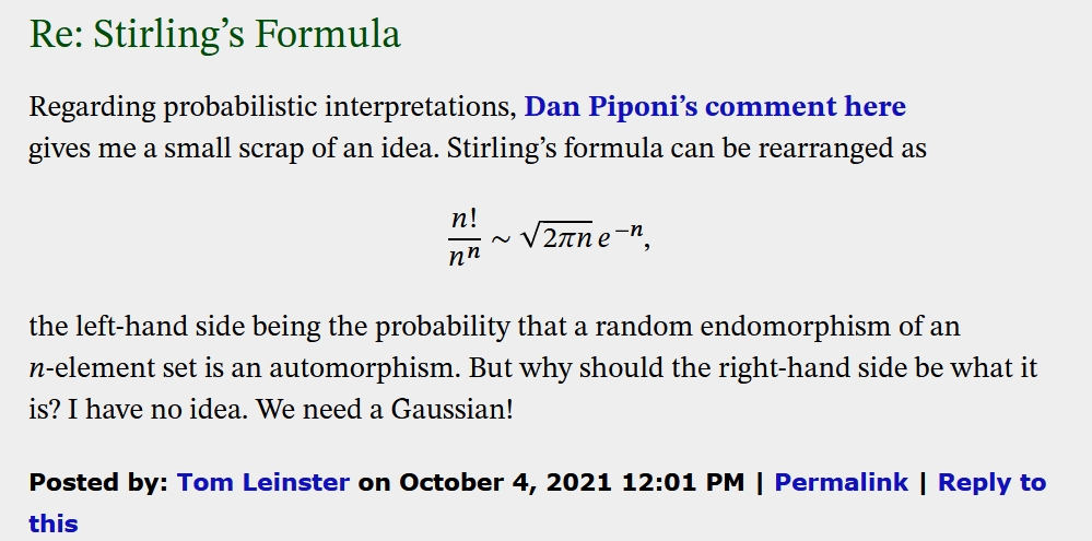
So I don't think we've gotten to the bottom of Stirling's formula! Comments at the n-Category Café contain other guesses about what it might 'really mean'. But they haven't crystallized yet.

October 7, 2021

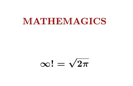
'Mathemagics' is a bunch of tricks that go beyond rigorous mathematics. Particle physicists use them a lot. Using a mathemagical trick called 'zeta function regularization', we can 'show' that infinity factorial is $\sqrt{2\pi }$.

This formula doesn't make literal sense, but we can write $$\ln (\mathrm{\infty }!)=\sum _{n=1}^{\mathrm{\infty }}\ln n.$$ This sum diverges, but $$\sum _{n=1}^{\mathrm{\infty }}{n}^{-s}\ln n$$ converges for $\mathrm{Re}(s)>1$ and we can analytically continue this function to $s=0$, getting $\frac{1}{2}\ln 2\pi$. So using this trick we can argue that $$\ln (\mathrm{\infty }!)=\frac{1}{2}\ln 2\pi ,$$ giving the equation above. Don't take it too seriously... but physicists use tricks like this all the time, and get results that agree with experiment.

To understand this trick we need to notice that $$\sum _{n=1}^{\mathrm{\infty }}{n}^{-s}\ln n=-\frac{d}{ds}\zeta (s)$$ where $$\zeta (s)=\sum _{n=1}^{\mathrm{\infty }}{n}^{-s}$$ is the definition of the Riemann zeta function for $\mathrm{Re}(s)>1$. But then — the hard part — we need to show we can analytically continue the Riemann zeta function to $s=0$, and get $${\zeta }^{\prime }(0)=-\frac{1}{2}\ln 2\pi$$ This last fact is a spinoff of Stirling's formula $$n!\sim \sqrt{2\pi n}{\left(\frac{n}{e}\right)}^n$$ So the mathemagical formula for $\mathrm{\infty }!$ is a crazy relative of this well-known, perfectly respectable asymptotic formula for $n!$.

To learn much more about this, read Cartier's article:

• Pierre Cartier, Mathemagics (a tribute to L. Euler and R. Feynman), Séminaire Lotharingien de Combinatoire 44 (2000), B44d.

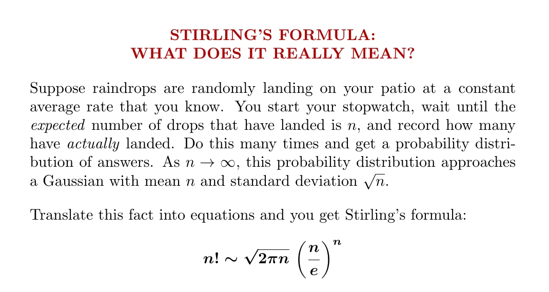
Stirling's formula for the factorial looks cool — but what does it really mean? This is my favorite explanation. You don't see the numbers $e$ and $2\pi$ in the words here, but they're hiding in the formula for a Gaussian probability distribution!

My description in words is informal. I'm really talking about a Poisson distribution. If raindrops land at an average rate $r$, this says that after time $t$ the probability of $k$ having landed is $$\frac{(rt{)}^k{e}^{-rt}}{k!}$$ This is where the factorial comes from.

At time $t$, the expected number of drops to have fallen is clearly $rt$. Since I said "wait until the expected number of drops that have landed is $n$", we want $rt=n$. Then the probability of $k$ having landed is $$\frac{n^k{e}^{-n}}{k!}$$

Next, what's the formula for a Gaussian with mean $n$ and standard deviation $\sqrt{n}$? Written as a function of $k$, it's

$$\frac{e^{-(k-n{)}^2/2n}}{\sqrt{2\pi n}}$$ If this matches the Poisson distribution above in the limit of large $n$, the two functions must match when $k=n$, at least asymptotically, so $$\frac{n^n{e}^{-n}}{n!}\sim \frac{1}{\sqrt{2\pi n}}$$ And this becomes Stirling's formula after a tiny bit of algebra!

I learned about this on Twitter: Ilya Razenshtyn showed how to prove Stirling's formula starting from probability theory this way. But it's much easier to use his ideas to check that my paragraph in words is a way of saying Stirling's formula.

October 13, 2021

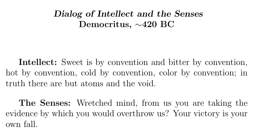
They called Democritus 'the laughing philosopher'. He not only came up with atoms: he explained how weird it is that science, based on our senses, has trouble explaining what it feels like to sense something.

And he did it in a way that would make a great comedy routine with two hand puppets.

By the way: a lot of my diary entries these days are polished versions of my tweets. Yesterday Dominic Cummings retweeted the above tweet of mine. He was chief advisor to Boris Johnson for about a year, and on Twitter he loves to weigh in on the culture wars, on the conservative side.

It's not as weird as when Ivanka Trump liked my tweet about rotations in 4 dimensions, but still it's weird. Or maybe not: Patrick Wintour in The Guardian reported that "Anna Karenina, maths and Bismarck are his three obsessions." But I wish some nice bigshots would like or retweet my stuff.

October 16, 2021

I love this movie showing a solution of the Kuramoto–Sivashinsky equation, made by Thien An. If you haven't seen her great math images on Twitter, check them out!

I hadn't known about this equation, and it looked completely crazy to me at first. But it turns out to be important, because it's one of the simplest partial differential equations that exhibits chaotic behavior.

As the image scrolls to the left, you're seeing how a real-valued function $u(t,x)$ of two real variables changes with the passage of time. The vertical direction is 'space', $x$, while the horizontal direction is time, $t$.

As time passes, bumps form and merge. I conjecture that they never split or disappear. This reflects the fact that the Kuramoto–Sivashinsky equation has a built-in arrow of time: it describes a world where the future is different than the past.

The behavior of these bumps makes the Kuramoto–Sivashinsky equation an excellent playground for thinking about how differential equations can describe 'things' with some individuality, even though their solutions are just smooth functions.

For much more on the Kuramoto–Sivashinsky conjecture, including attempts to make my conjecture precise and my work with Steve Huntsman and Cheyne Weis to get numerical evidence for it, read these:

• John Baez, The Kuramoto–Sivashinsky equation (part 1).
• John Baez, The Kuramoto–Sivashinsky equation (part 2).

Another nice illusion by Akioyishi Kitaoka.

October 29, 2021

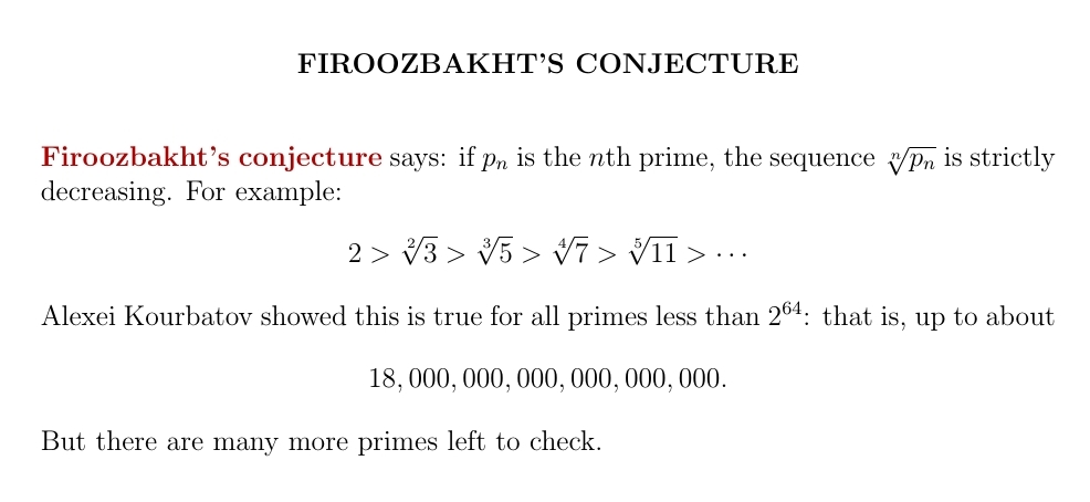
The Iranian mathematician Farideh Firoozbakht made a strong conjecture in 1982: the $n$th root of the $n$th prime keeps getting smaller as we make $n$ bigger! It's been checked for primes up to about 18 quintillion, but nobody has a clue how to prove it. In fact, some experts think it's probably false.

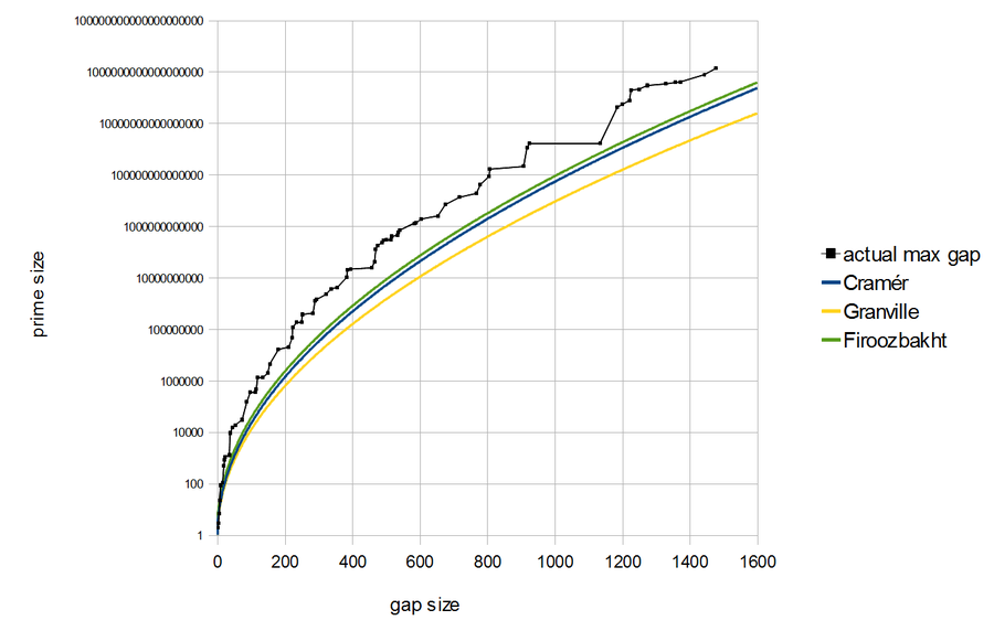
Firoozbakht's conjecture says the gaps between primes don't get too big too fast. As you can see here, it's stronger than Cramér's or Granville's conjectures on prime gaps — and it gets scarily close to being wrong at times, like when the largest prime gap jumps from 924 to 1132 at the prime 1693182318746371 — you can see that big horizontal black line above.

Farideh Firoozbakht checked her conjecture up to about 4 trillion using a table of large gaps between primes: those are what could make the conjecture false. In 2015 Alexei Kourbatov checked it up to 4 quintillion, in this paper here:

• Alexei Kourbatov, Verification of the Firoozbakht conjecture for primes up to four quintillion, International Mathematical Forum 10 (2015), 283–288.

• Alexei Kourbatov, The Firoozbakht conjecture.

If true, Firoozbakht's conjecture will imply a lot of good stuff, listed in this paper by Ferreira and Mariano:

• Luan Alberto Ferreira and Hugo Luiz Mariano, Some consequences of the Firoozbakht's conjecture.

It's known that the Riemann Hypothesis implies the $n$th prime gap is eventually less than $\sqrt{p_n}\ln p_n$, where $p_n$ is the $n$th prime. Firoozbakht's conjecture implies something much stronger: it's eventually less than $c(\ln p_n{)}^2$, where you can choose $c$ to be any constant bigger than 1. This is Theorem 2.2 in Ferreira and Mariano's paper.

Nobody knows how to prove Firoozbakht's conjecture using the Riemann Hypothesis. But conversely, it seems nobody has shown Firoozbakht implies Riemann!

There are even some good theoretical reasons for believing Firoozbakht's conjecture is false! Granville has a nice probabilistic model of the behavior of primes that predicts that there are infinitely many gaps over $1.1(\ln p_n{)}^2$ in width. Firoozbakht's conjecture, on the other hand, implies they eventually all get smaller than this, as I mentioned above.

For more on Granville's probabilistic model of prime and its consequences for the largest prime gaps, see:

• Terry Tao, Large prime gaps and probabilistic models, What's New, August 26, 2019.

Farideh Firoozbakht, alas, died in 2019 at the age of 57. She studied pharmacology and later mathematics at the University of Isfahan and later taught mathematics at that university. That, and her conjecture, is all I know about her. I wish I could ask her how she came up with her conjecture, and ask her a bit about what her life was like.

If anyone knows, please tell me!

I thank Maarten Morier for telling me about Firoozbakht's conjecture.

For my November 2021 diary, go here.

home