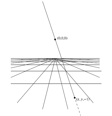
Projective geometry is a venerable subject that has its origins in the study of perspective by Renaissance painters. As seen by the eye, parallel lines — e.g., train tracks — appear to meet at a 'point at infinity'. When one changes ones viewpoint, distances and angles appear to change, but points remain points and lines remain lines. These facts suggest a modification of Euclidean plane geometry, based on a set of points, a set of lines, and relation whereby a point 'lies on' a line, satisfying the following axioms:
We have already met one example of a projective plane in Section
2.1: the smallest one of all, the Fano plane. The example
relevant to perspective is the real projective plane, ![]() . Here the
points are lines through the origin in
. Here the
points are lines through the origin in ![]() , the lines are planes
through the origin in
, the lines are planes
through the origin in ![]() , and the relation of 'lying on' is taken to
be inclusion. Each point
, and the relation of 'lying on' is taken to
be inclusion. Each point
![]() determines a point in
determines a point in
![]() , namely the line in
, namely the line in ![]() containing the origin and the point
containing the origin and the point
![]() :
:
There are also other points in ![]() , the 'points at infinity',
corresponding to lines through the origin in
, the 'points at infinity',
corresponding to lines through the origin in ![]() that do not
intersect the plane
that do not
intersect the plane ![]() . For example, any point on the
horizon in the above picture determines a point at infinity.
. For example, any point on the
horizon in the above picture determines a point at infinity.
Projective geometry is also interesting in higher dimensions. One can define a projective space by the following axioms:
If ![]() is any field, there is an
is any field, there is an ![]() -dimensional projective space
called
-dimensional projective space
called ![]() where the points are lines through the origin in
where the points are lines through the origin in
![]() , the lines are planes through the origin in
, the lines are planes through the origin in ![]() , and
the relation of 'lying on' is inclusion. In fact, this construction
works even when
, and
the relation of 'lying on' is inclusion. In fact, this construction
works even when ![]() is a mere skew field: a ring such that every
nonzero element has a left and right multiplicative inverse. We just
need to be a bit careful about defining lines and planes through the
origin in
is a mere skew field: a ring such that every
nonzero element has a left and right multiplicative inverse. We just
need to be a bit careful about defining lines and planes through the
origin in ![]() . To do this, we use the fact that
. To do this, we use the fact that ![]() is a
is a
![]() -bimodule in an obvious way. We take a line through the origin to
be any set
-bimodule in an obvious way. We take a line through the origin to
be any set
Given this example, the question naturally arises whether every
projective ![]() -space is of the form
-space is of the form ![]() for some skew field
for some skew field ![]() .
The answer is quite surprising: yes, but only if
.
The answer is quite surprising: yes, but only if ![]() . Projective
planes are more subtle [84]. A projective plane comes
from a skew field if and only if it satisfies an extra axiom, the
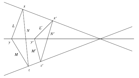
'axiom of Desargues', which goes as follows. Define a triangle
to be a triple of points that don't all lie on the same line. Now,
suppose we have two triangles
. Projective
planes are more subtle [84]. A projective plane comes
from a skew field if and only if it satisfies an extra axiom, the
'axiom of Desargues', which goes as follows. Define a triangle
to be a triple of points that don't all lie on the same line. Now,
suppose we have two triangles ![]() and
and ![]() . The sides of each
triangle determine three lines, say
. The sides of each
triangle determine three lines, say ![]() and
and ![]() . Sometimes
the line through
. Sometimes
the line through ![]() and
and ![]() , the line through
, the line through ![]() and
and ![]() , and
the line through
, and
the line through ![]() and
and ![]() will all intersect at the same point:
will all intersect at the same point:
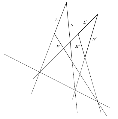
The axiom of Desargues says that whenever this happens, something else happens: the intersection of
This axiom holds automatically for projective spaces of dimension 3 or more, but not for projective planes. A projective plane satisfying this axiom is called Desarguesian.
The axiom of Desargues is pretty, but what is its connection to skew
fields? Suppose we start with a projective plane ![]() and try to
reconstruct a skew field from it. We can choose any line
and try to
reconstruct a skew field from it. We can choose any line ![]() , choose
three distinct points on this line, call them
, choose
three distinct points on this line, call them ![]() , and
, and ![]() , and
set
, and
set
![]() . Copying geometric constructions that work
when
. Copying geometric constructions that work
when ![]() , we can define addition and multiplication of points in
, we can define addition and multiplication of points in
![]() . In general the resulting structure
. In general the resulting structure
![]() will not
be a skew field. Even worse, it will depend in a nontrivial way on the
choices made. However, if we assume the axiom of Desargues, these
problems go away. We thus obtain a one-to-one correspondence between
isomorphism classes of skew fields and isomorphism classes of
Desarguesian projective planes.
will not
be a skew field. Even worse, it will depend in a nontrivial way on the
choices made. However, if we assume the axiom of Desargues, these
problems go away. We thus obtain a one-to-one correspondence between
isomorphism classes of skew fields and isomorphism classes of
Desarguesian projective planes.
Projective geometry was very fashionable in the 1800s, with such
worthies as Poncelet, Brianchon, Steiner and von Staudt making important
contributions. Later it was overshadowed by other forms of geometry.
However, work on the subject continued, and in 1933 Ruth Moufang
constructed a remarkable example of a non-Desarguesian projective plane
using the octonions [69]. As we shall see, this projective
plane deserves the name ![]() .
.
The 1930s also saw the rise of another reason for interest in projective
geometry: quantum mechanics! Quantum theory is distressingly different
from the classical Newtonian physics we have learnt to love. In
classical mechanics, observables are described by real-valued functions.
In quantum mechanics, they are often described by hermitian ![]() complex matrices. In both cases, observables are closed under
addition and multiplication by real scalars. However, in quantum
mechanics, observables do not form an associative algebra. Still,
one can raise an observable to a power, and from squaring one
can construct a commutative but nonassociative product:
complex matrices. In both cases, observables are closed under
addition and multiplication by real scalars. However, in quantum
mechanics, observables do not form an associative algebra. Still,
one can raise an observable to a power, and from squaring one
can construct a commutative but nonassociative product:
In 1934, Jordan published a paper with von Neumann and Wigner
classifying all formally real Jordan algebras [55]. The
classification is nice and succinct. An ideal in the Jordan algebra
![]() is a subspace
is a subspace ![]() such that
such that ![]() implies
implies
![]() for all
for all ![]() . A Jordan algebra
. A Jordan algebra ![]() is simple if its
only ideals are
is simple if its
only ideals are ![]() and
and ![]() itself. Every formally real Jordan
algebra is a direct sum of simple ones. The simple formally real Jordan
algebras consist of 4 infinite families and one exception.
itself. Every formally real Jordan
algebra is a direct sum of simple ones. The simple formally real Jordan
algebras consist of 4 infinite families and one exception.
The paper by Jordan, von Neumann and Wigner appears to have been
uninfluenced by Moufang's discovery of ![]() , but in fact they are
related. A projection in a formally real Jordan algebra is
defined to be an element
, but in fact they are
related. A projection in a formally real Jordan algebra is
defined to be an element ![]() with
with ![]() . In the familiar case of
. In the familiar case of
![]() , these correspond to hermitian matrices with eigenvalues
, these correspond to hermitian matrices with eigenvalues ![]() and
and ![]() , so they are used to describe observables that assume only two
values — e.g., 'true' and 'false'. This suggests treating projections
in a formally real Jordan algebra as propositions in a kind of 'quantum
logic'. The partial order helps us do this: given projections
, so they are used to describe observables that assume only two
values — e.g., 'true' and 'false'. This suggests treating projections
in a formally real Jordan algebra as propositions in a kind of 'quantum
logic'. The partial order helps us do this: given projections ![]() and
and
![]() , we say that
, we say that ![]() 'implies'
'implies' ![]() if
if ![]() .
.
The relation between Jordan algebras and quantum logic is already
interesting [30], but the real fun starts when we note
that projections in ![]() correspond to subspaces of
correspond to subspaces of ![]() . This
sets up a relationship to projective geometry [91], since
the projections onto 1-dimensional subspaces correspond to points in
. This
sets up a relationship to projective geometry [91], since
the projections onto 1-dimensional subspaces correspond to points in
![]() , while the projections onto 2-dimensional subspaces correspond
to lines. Even better, we can work out the dimension of a subspace
, while the projections onto 2-dimensional subspaces correspond
to lines. Even better, we can work out the dimension of a subspace
![]() from the corresponding projection
from the corresponding projection
![]() using only the partial order on projections:
using only the partial order on projections: ![]() has dimension
has dimension ![]() iff
the longest chain of distinct projections
iff
the longest chain of distinct projections
If we try this starting with ![]() ,
, ![]() or
or ![]() , we
succeed when
, we
succeed when ![]() , and we obtain the projective spaces
, and we obtain the projective spaces ![]() ,
,
![]() and
and ![]() , respectively. If we try this starting with the
spin factor
, respectively. If we try this starting with the
spin factor
![]() we succeed when
we succeed when ![]() , and obtain a
series of 1-dimensional projective spaces related to Lorentzian
geometry. Finally, in 1949 Jordan [54] discovered that if we
try this construction starting with the exceptional Jordan algebra, we
get the projective plane discovered by Moufang:
, and obtain a
series of 1-dimensional projective spaces related to Lorentzian
geometry. Finally, in 1949 Jordan [54] discovered that if we
try this construction starting with the exceptional Jordan algebra, we
get the projective plane discovered by Moufang: ![]() .
.
In what follows we describe the octonionic projective plane
and exceptional Jordan algebra in more detail. But first let us
consider the octonionic projective line, and the Jordan algebra
![]() .
.
© 2001 John Baez